Are you tired of scrolling through endless rows and columns in Excel? We’ve got you covered!
In this article, we’ll show you how to freeze rows and columns in Excel, making your data analysis a breeze. Say goodbye to losing track of important information and hello to a more efficient way of working.
So grab your mouse and get ready to learn the tricks and techniques to master this essential Excel skill. Let’s dive in!
Understanding the Importance of Freezing Rows and Columns
You’ll want to understand why freezing rows and columns is important in Excel.
When working with large data sets, it can become overwhelming to navigate through rows and columns that constantly move out of sight. Freezing rows and columns allows you to keep important information visible no matter how far you scroll.
This is especially useful when working with headers or labels that you need to reference frequently. By freezing these rows or columns, you can easily locate and compare data without losing your place.
Additionally, freezing rows and columns can help maintain consistency and prevent errors when working with formulas or sorting data. It provides a fixed reference point that remains visible, making your Excel experience more efficient and organized.
Step-by-Step Guide to Freezing Rows in Excel
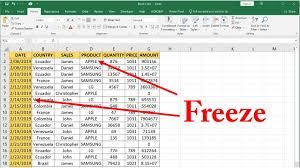
To keep specific information visible while scrolling in Excel, it’s as simple as selecting the desired rows and locking them in place.
First, open your Excel spreadsheet and locate the row you want to freeze. Click on the row number to select the entire row.
Next, go to the ‘View’ tab in the toolbar and click on ‘Freeze Panes.’ From the dropdown menu, select ‘Freeze Panes’ again.
You will notice a faint line appear below the frozen row, indicating that it has been successfully locked in place.
Now, when you scroll through your spreadsheet, the frozen row will always stay visible at the top of the window. This is incredibly useful when working with large datasets or when you need to reference specific information while navigating through your Excel file.
Mastering the Art of Freezing Columns in Excel
When working with large datasets in Excel, it’s helpful to ensure that specific information remains visible while scrolling. Freezing columns in Excel allows you to keep important data in view even when you navigate through the spreadsheet.
To freeze columns, start by selecting the column to the right of the ones you want to freeze. Then, go to the ‘View’ tab and click on ‘Freeze Panes’. From the drop-down menu, select ‘Freeze Panes’ again. You will notice a thin gray line appear on the left side of the selected column. This indicates that the columns to the left of the line are frozen.
Now, when you scroll horizontally, those columns will remain visible, providing you with easy access to the crucial data you need.
Tips and Tricks for Efficiently Freezing Rows and Columns
One useful trick for efficiently freezing rows and columns in Excel is to use the keyboard shortcut Ctrl + Shift + F5. This shortcut brings up the ‘Go To’ dialog box, where you can select specific cells or ranges to navigate to.
To freeze rows and columns, first select the cell where you want the freezing to begin. Then, press Ctrl + Shift + F5 to bring up the dialog box.
Next, click on the ‘Special’ button, and select ‘Constants’ from the list. Check the box next to ‘Constants’ and click ‘OK’. This will select all the cells containing constants in your worksheet.
Advanced Techniques for Customizing Frozen Rows and Columns in Excel
Customizing frozen rows and columns in Excel becomes more advanced as you explore different options and settings.
To further enhance your Excel experience, you can adjust the frozen pane size and position. Simply go to the View tab, click on Freeze Panes, and select Freeze Panes again. This will allow you to manually adjust the size and position of the frozen pane by dragging the borders.
Another advanced technique is freezing multiple rows or columns. To do this, select the row or column below or to the right of the rows or columns you want to freeze. Then, go to the View tab, click on Freeze Panes, and select Freeze Panes again. This will freeze all the rows above or columns to the left of your selection, giving you a customized frozen view.
Conclusion
In conclusion, freezing rows and columns in Excel is a valuable skill that can greatly enhance your data management and analysis.
By understanding the importance of freezing, following the step-by-step guide, and mastering the art of freezing columns, you can efficiently navigate through large spreadsheets.
Additionally, by utilizing tips and tricks and exploring advanced techniques, you can customize your frozen rows and columns to suit your specific needs.
With these skills, you’ll be able to work with Excel more effectively and improve your productivity.