Are you tired of scrolling through your Excel spreadsheet and losing track of the top row? Look no further!
This article will show you how to freeze the top row in Excel, ensuring that it stays visible no matter how far you scroll.
With a step-by-step guide, you’ll learn the most efficient methods to freeze the top row and discover useful tips and tricks along the way.
Say goodbye to the hassle of losing sight of important information in your spreadsheet – let’s get started!
Understanding the Importance of Freezing the Top Row in Excel
To better navigate through your Excel spreadsheet, it’s important for you to understand why you should freeze the top row.
Freezing the top row allows you to keep important column headers visible as you scroll down the sheet. This can be particularly helpful when working with large datasets or when analyzing data.
By freezing the top row, you can easily refer to the column headers without having to constantly scroll back to the top of the sheet. It saves you time and effort, making your work more efficient.
Additionally, freezing the top row helps maintain context and prevents confusion while working with multiple rows of data. It ensures that you always know which data belongs to which column, enhancing the overall organization and clarity of your spreadsheet.
Step-by-Step Guide to Freezing the Top Row in Excel
Take a moment to ensure that you can always see the first row of your spreadsheet in Excel. Freezing the top row in Excel is a helpful feature that allows you to keep the header row visible as you scroll through your data.
To freeze the top row, click on the View tab at the top of the Excel window. In the Window group, you will find the Freeze Panes option. Click on it and select ‘Freeze Top Row.’
Once you do this, the top row will remain fixed in place, no matter how far down you scroll. This makes it easy to refer to the column headers or any other important information in the first row while working with large datasets.
Exploring Different Methods to Freeze the Top Row in Excel
There are various techniques you can use to keep the first row visible in Excel.
One method is to use the Freeze Panes feature. To do this, you need to select the row below the one you want to freeze, then go to the View tab and click on Freeze Panes.
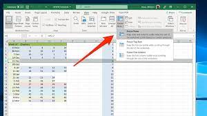
Another option is to use the Split feature. Simply click on the cell below the row you want to freeze, go to the View tab, and click on Split. This will create a horizontal split, keeping the top row visible at all times.
Lastly, you can also use the Window tab to split the worksheet into two separate windows. This way, you can have the first row visible in one window while scrolling through the rest of the sheet in the other window.
Tips and Tricks for Efficiently Using the Freeze Top Row Feature in Excel
When using the Freeze Panes feature in Excel, you can easily keep the first row visible at all times. This is especially useful when you have a large dataset and want the column headers to remain visible while scrolling through the rest of the worksheet.
To freeze the top row, simply select the row below the one you want to freeze. For example, if you want to freeze the first row, select cell A2. Then, go to the View tab, click on Freeze Panes, and select Freeze Panes from the drop-down menu.
Now, when you scroll down, the top row will remain fixed at the top of the screen, allowing you to easily reference the column headers as you work with your data.
Common Issues and Troubleshooting Tips for Freezing the Top Row in Excel
If you’re having trouble with the first row staying visible in Excel, one possible solution is to adjust the cell range you have selected before freezing the panes.
Sometimes, when you freeze the top row, Excel automatically selects the whole sheet as the cell range, causing the first row to disappear. To fix this, you can manually select the range of cells you want to freeze before applying the freeze panes feature.
Simply click on the cell below the row you want to freeze, and then drag your cursor to the right until you reach the last column you want to include in the frozen area. This will ensure that only the selected cells are frozen, and the first row will remain visible as you scroll through your spreadsheet.
Conclusion
In conclusion, now that you know how to freeze the top row in Excel, you can improve your data analysis and organization skills. By keeping the header row visible while scrolling through large datasets, you can easily identify and understand the data in each column.
Remember to use the step-by-step guide and explore different methods to find the one that works best for you. With these tips and tricks, you’ll be able to efficiently use the freeze top row feature in Excel and troubleshoot any issues that may arise.
Happy Excel-ing!