Are you tired of continuously scrolling through your Google Sheets to reference important information at the top?
In this article, we will show you how to freeze rows in Google Sheets, making your data easily accessible no matter where you are in the spreadsheet.
By following our step-by-step guide and utilizing advanced techniques, you’ll be able to save time and increase productivity.
Say goodbye to endless scrolling and hello to a more efficient way of working with Google Sheets.
Why Is It Important to Freeze Rows in Google Sheets
You should freeze rows in Google Sheets because it allows you to keep important information visible while scrolling through your spreadsheet. When you have a large dataset or multiple columns, it can become difficult to keep track of important data as you navigate through the sheet.
Freezing rows ensures that you always have access to the most crucial information, even as you scroll down. For example, if you have column headers or a summary row at the top of your sheet, freezing those rows will keep them in place, no matter how far down you scroll. This makes it easier to analyze and interpret your data without constantly having to scroll back up.
Freezing rows in Google Sheets is a simple yet effective way to enhance your productivity and streamline your work process.
The Benefits of Freezing Rows in Google Sheets
One of the advantages of freezing rows in Google Sheets is that it allows for easier navigation and organization of data. When you freeze rows, you can keep important information, such as headers or labels, visible at all times, even when scrolling through a large spreadsheet.
This is especially helpful when working with a lot of data, as it saves you from constantly having to scroll back up to see what each column represents. By freezing rows, you can also easily compare data in different sections of your spreadsheet without losing track of the headers.
This feature improves efficiency and productivity, as it reduces the time and effort required to locate and reference specific information. So, take advantage of freezing rows in Google Sheets and make your data management a breeze.
Step-By-Step Guide to Freezing Rows in Google Sheets
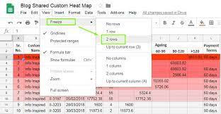
To freeze specific sections of your spreadsheet, simply navigate to the ‘View’ tab and select the ‘Freeze’ option. This feature in Google Sheets is incredibly useful when you want to keep certain rows visible while scrolling through your data.
Here’s a step-by-step guide to help you freeze rows in Google Sheets.
- First, open your spreadsheet and click on the ‘View’ tab at the top of the screen.
- Next, select the ‘Freeze’ option from the drop-down menu.
- A new menu will appear with different freeze options. Choose the ‘Freeze x rows’ option, where ‘x’ represents the number of rows you want to freeze.
- Finally, click on the row number below the last row you want to freeze, and voila! Your selected rows will now remain visible as you scroll through your spreadsheet.
Advanced Techniques for Freezing Rows in Google Sheets
If you want a more advanced way to keep certain sections visible while scrolling through your data in Google Sheets, consider using the freeze feature.
This feature allows you to freeze not only rows, but also columns, making it easier to navigate through large spreadsheets.
To freeze rows and columns simultaneously, simply select the cell below the row you want to freeze and to the right of the column you want to freeze.
Then, go to the ‘View’ tab and click on ‘Freeze’.
You can also choose to freeze multiple rows or columns by selecting the appropriate cells before freezing.
This advanced technique is especially useful when working with complex data or when you need to refer to specific information while scrolling through your spreadsheet.
Troubleshooting Common Issues When Freezing Rows in Google Sheets
When troubleshooting freezing issues in Google Sheets, it’s important to check for any conflicting formatting or merged cells that could be causing the problem.
Sometimes, when you try to freeze rows, you may encounter unexpected freezing behavior. One common issue is conflicting formatting. If you have different formatting applied to the same range of cells, it can cause conflicts and prevent freezing from working correctly.
Another issue to look out for is merged cells. When cells are merged, it can disrupt the freezing functionality. To fix this, you need to unmerge the cells and try freezing rows again.
Conclusion
In conclusion, freezing rows in Google Sheets is a valuable feature that can greatly enhance your spreadsheet experience. By keeping important information visible as you scroll, you can easily navigate through large amounts of data without losing context.
This simple yet powerful technique can save you time and effort, allowing you to focus on analyzing and interpreting your data. So go ahead and start freezing those rows in Google Sheets to optimize your workflow and make your spreadsheet tasks more efficient.